I’ve been boggled by this question in the topic ever since I
got absorbance readings on an ELISA test kit >2, up to Absorbance units of
3.5 and so on.
I speculated how it could be possible, and with George’s
explanation came up with all sorts of theories that plate readers probably
correct for the light path etc.
In my mind, since the formula for absorbance is the following: Abs = 2 – log (%T), my thoughts were that it is impossible to have absorbance values more than 2. Hence I thought Abs. should be discarded above 2.
I have however seen on this page,
which explained it quite well with a table, that it is indeed possible to
obtain absorbance values >2 if the light source is strong enough and the
spectrophotometer is sensitive enough to obtain accurate readings in this
range.
The theory is however, when the transmittance of <1% happens, log part of the formula (log%T), becomes a negative value. One thus subtracts a minus, theoretically making absorbances possible to indefinite values.
Absorbance (optical density)
Transmittance %
0
100
1
10
2
1
3
0.1
4
0.01
5
0.001
6
0.0001
“At an absorbance of 6, only one 10,000th of one percent of a particular wavelength is being transmitted through the filter (lens). Absorbance is measured with a spectrophotometer, which establishes the light transmission and calculates the absorbance. However, the spectrophotometer can only measure absorbance up to 4.5 directly. Beyond this level all values must be extrapolated. For example, if a 2 mm thick filter is measured to have an absorbance of 3, then it is assumed that a 4 mm thick filter should have an absorbance of 6.”
Obviously there are still limitations to this and the general principle remains that absorbance units should be sought to be <1.8 (actually ideally now that I think of it <1.0) to make the standards and measurements more in the linear range (i.e. %Transmittance less than (100-10^10)=<90), for Abs. <1. I do think however that spectrophotometers (and plate readers in particular) these days are probably more sensitive than historically and hence one could go up a bit with the absorbance, given the understanding of the limitations regarding imprecision at these Absorbance levels.
One should understand that the absorbance >2 units does measure light intensity at a %Transmittance value between 99% and 100%, hence the room for error becomes exponentially bigger if the spectrophotometer’s CV is not precise enough at these %T values.
Still to be revealed to me is the fact that absorbance
values I obtained in Spectrophotometers and plate readers often did not
correlate well, even when correcting for the light path length, and I would
probably just need to read more to get proper clarity, or the path length
through the well in the plate reader was not accurately measured by me.
One way to correct for path length of water could be to measure the absorbance
of the water / solvent at 977nm (infrared; IR) and correct therefor, but most
specs we use don’t have IR measuring capabilities.
Albumin Assay – Bromocresol Green method
Practical Documentation:
Aims
To perform serum albumin determinations on samples, explain the principle behind the Bromocresol Green method for albumin measurement and to list the factors that will cause interference with this method.
Principle
Albumin is known for its ability to bind many types of organic compounds, including organic dyes. When albumin selectively binds with Bromcresol Green (BCG) it causes a change in the absorbance maximum of BCG. The intense blue-green complex that is formed has an absorbance max of 670nm. Bromocresol reagent at pH 4.3 is negatively charged. The pI of albumin is 4.7.
For all spectrometric assays, always use a Reagent
blank. It usually contains all diluents and reagent in the reaction
solution, but no sample. Some reagent blanks do contain the sample as well, but
they lack one crucial reagent component needed to produce a colour-yielding
reaction. This is different from the water used to zero a spectrophotometer
(set 100% T).
Generate a calibration curve of
at least 8 standards (0- 80 g/L) by diluting the Albumin Stock (100 g/L).
In labelled tubes, set up a
calibration, controls and test samples as follows:
Sample
Water (µL)
Std (µL)
Control (µL)
Sample (µL)
BCG Reagent (µL)
Blank
310
–
–
–
300
Calibrators
300
10
–
–
300
Control
300
–
10
–
300
Serum Sample
300
–
–
10
300
Figure 1. Setting up the standards for the calibration curve.
To set up a standard curve with more points along the usable range, I chose more points in the concentration range 20 – 40 g/L, which in my experience constitutes the bulk of albumin measurements.
3. Mix well read immediately at 630nm and record absorbances
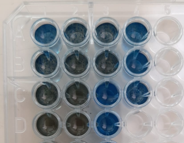
Layout of wells
Dilution as per manual
Dilution of 1:2 with H2O
1
2
3
4
A
Standard 0
Unknown 1
Standard 0
Unknown 1
B
Standard 1
Unknown 2
Standard 1
Unknown 2
C
Standard 2
Unknown 3
Standard 2
Unknown 3
D
Standard 3
Unknown 4
Standard 3
Unknown 4
E
Standard 4
Unknown 5
Standard 4
Unknown 5
F
Standard 5
QC Low
Standard 5
QC Low
G
Standard 6
QC High
Standard 6
QC High
H
Standard 7
Standard 7
Layout of wellsLayout of wells
Absorbance
Absorbance
Standard concentration (g/L)
No dil
Dil 1:2 (150uL reagent mix + 150uL H2O
0
0.095
0.065
20
0.506
0.245
25
0.719
0.345
30
0.779
0.395
35
0.784
0.411
40
0.999
0.504
50
1.242
0.593
80
1.477
0.68
4. Plot a standard curve and determine experimental concentrations of controls and serum samples
Figure 2 – Deriving the formula was done with a statistical Calculator by entering the respective X- and Y-values into a table and obtaining a slope and y-intercept by linear regression. Only the neat reagent mix’s formula was done manually with a calculator. Slope (b) was calculated to be 0.01769 and y-intercept (a) was 0.206. These values corresponded to the values when plotting an X-Y plot on Microsoft Excel (see 2 standard curve data plots above).
The figure below illustrates the formula used to determine the unknown concentrations.
Unknown concentrations were calculated as follows:
Unknowns Sample no.
Absorbance
Absorbance (Diluted 1:2)
Calculated concentration
Calculated concentration (Diluted 1:2)
Reference albumin values (from Roche Cobas 6000)
1
0.893
0.48
Hemolysed
38.8
44.2
29.1
2
1.057
0.55
48.1
53.0
44.2
3
0.614
0.334
23.1
26.0
22
4
0.997
0.5
Hemolysed
44.7
46.7
38.6
5
0.894
0.479
38.9
44.1
33.2
Lo
0.843
0.453
36.0
40.9
31.9
Hi
1.161
0.593
54.0
58.4
49.4
Compare results to expected results and comment on any differences between the manual BCG vs automated BCP assays.
Figure 3 – Manual BCG method vs. Automated BCP method (Roche). It can be seen that the manual BCG method overestimated the albumin concentration in all serum samples. A possible explanation for this difference is: 1. Pipetting error 2. Interferring substances in the serum which absorb light at 670nm. 3. It may be due to the fact that albumin stock solution was made up with water as opposed to physiological albumin-free serum matrix. 4. Hemolysis – Evidenced by one of the hemolysed samples which clearly measured falsely high.
A haemolysed sample is brought to the laboratory for albumin analysis. Can the sample be used? Discuss.
Yes. Hemoglobin does not absorb light at 670 nm, therefor will not interfere significantly with the analysis. See figure below:
It does however interfere in the following manner:
Hemoglobin decreases the apparent albumin concentration by 1 g/L for each 100 g/L added. Blanking does not correct this interference, and the negative bias is therefore caused by interference with the dye binding rather than hemoglobin color. For the BCP method, a blank correction is required on icteric sera and on grossly hemolyzed and grossly lipemic sera to correct for an underestimation of albumin caused by these agents. Heparin causes a positive interference with BCP and BCG methods. This interference can be eliminated by the addition of hexadimethrine bromide to a concentration of 50 mg/L in the BCP reagent
Kaplan’s Methods
Why is it not desirable to incubate the reaction before measuring the absorbance?
Incubating the sample can give rise to other non-specific binding of analytes in the sample to the chromophore dye and a falsely elevated reading can be obtained.
Some analyzers can measure the absorbance of the BCG reaction within 30 seconds after adding sample. Does this tend to increase the specificity of the reaction?
Yes. The less time there is for other interfering substances to bind to BCG, potentially the more specific it will be to albumin, as albumin is the more specific binding to BCG.
Probably the most promising adaptation of the BCG reaction for albumin analysis utilizes fast reaction readings. Gustafsson reported that measuring the absorbance of the BCG-protein complex at 629 nm at a time shortly after mixing improves the specificity of the assay. Interference by other proteins such as ceruloplasmin and orosomucoid becomes significant at times greater than 5 minutes.
Kaplan’s Methods
Total Protein assay – Bradford
Practical 3 : PROTEIN ASSAY- BRADFORD Total /100
INTRODUCTION The Bradford protein assay, is a spectrophotometric assay that is more popular for protein concentration determination than other known protein assay such as the Lowry assay. The Bradford assay is simple, more sensitive and faster than other protein assays (Kruger, 2009). This assay is an example of a dye-binding assay and the dye used is Coomassie Brilliant Blue G-250 (Bradford, 1976; Becker, Caldwell and Zachgo, 1996; Kruger, 2009; Nouroozi and Noroozi, Moulood Valipour Ahmadizadeh, 2015). The principle of this assay relies on the physical interaction of the dye and protein in solution and results in an observable change in colour. The colour change is as follows; red (Amax 465 nm), when not bound to proteins and blue (Amax 595 nm) form of the dye carries a (-) charge and interacts with (+) charges on proteins to form a complex (Becker, Caldwell and Zachgo, 1996).
OBJECTIVES 2.1. To prepare standards through a series of dilutions 2.2. To measure the unknown concentration of a protein in solution via a spectrophotometer 2.3. To analyse, interpret results about CV%, SD, LOD and LOQ.
PROCEDURES A. PREPARATION BEFORE THE PRACTICAL Complete the following BEFORE your practical session: • You would need to do some extra reading on the Bradford protein assay and spectrophotometer principles (i.e. Beer Lambert law) in preparation for your practical and test. • Find and print SDS’s for the following chemicals; Tris (trisaminomethane), Hidrochloric acid (HCL), ethanol, Phosphoric acid and Coomassie Brilliant Blue G-250. • Prepare a practical plan for your experiment that you will be conducting today.
B. PRACTICAL SESSION (Total 50) Complete the following DURING your practical session: (1) Complete the practical test. (2) Using the Bradford Assay determine as follows: Materials provided: • Tris buffer: 10 mM Tris-HCl (pH 7.0)] • Bovine serum albumin (BSA) stock solution: [2 mg/ml BSA in Tris buffer (pH 7)] • Bradford reagent; [0.01% (w/v) Coomassie Brilliant Blue G-250, 4.7% (w/v) ethanol, 8.5% (w/v) phosphoric acid] • Unknown protein sample
Method: a) In Eppendorf tubes, prepare a series of BSA solutions of varying concentration by diluting the 2 mg/ml BSA stock solution with Tris-HCL buffer (You will need ~200μL of each dilution) to set up a calibration curve (at least 7 concentrations to be used).
Serial dilutions were made in 1.5mL Eppendorf tubes:
Standard no.
Protein concentration (ug/ml)
1 (500uL of provided 2ug/ml stock solution)
2
2 (250 uL of S1 plus 250uL Tris-HCl diluent)
1
3 (250 uL of S2 plus 250uL Tris-HCl diluent)
0.5
4 (250 uL of S3 plus 250uL Tris-HCl diluent)
0.25
5 (250 uL of S4 plus 250uL Tris-HCl diluent)
0.125
6 (250 uL of S5 plus 250uL Tris-HCl diluent)
0.0625
7 (250 uL of S6 plus 250uL Tris-HCl diluent)
0.03125
8 (Also Blank – Only 250uL Tris-HCl)
0
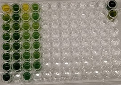
Standard preparations.
b) Add 2.5 mL of Bradford reagent to a separate cuvette for each of your samples and label them appropriately. Consider the value of determining the concentration of one or more dilutions of your unknown sample as well as the undiluted (“neat”) unknown sample.
To save cuvettes, I have used an old refurbished microtitre plate with 10x less volume, hence 250uL
c) Prepare your samples by adding 50μL of each protein sample (diluted standard or unknown) separately to the Bradford reagent in the appropriately labelled tube. Mix the tubes by gentle inversion several times, and let the colour develop for 5 min. Observe and record the colour change of your standard samples as a function of protein concentration. A blank sample is prepared by mixing 50μL Tris buffer with 2.5 ml Bradford reagent.
As above, to save reagent and test my pipetting skills, I have used 5uL as one set of additions and also made a 1:1 (2x) dilution of my standards to run another calibration curve. The unknown sample was also added as neat and a 2x dilution.
d) You will need to determine which portion of the UV/vis spectrum, specifically which wavelength will be useful for following the dye bound by protein. Take a full spectral scan of your Bradford reagent blank. When your standard samples have fully developed, take a full spectral scan of the most concentrated standard you prepared.
Fig. 1 – Wavelength scan of the reagent blank as well as the Highest standard after full colour development.
e) Based on your results, choose a single wavelength suitable to analyse the results of your dye-binding assay. Measure and record the absorbance of each standard and unknown sample at your chosen wavelengths using cuvettes.
From above wavelength scan it is evidenced that the maximum absorbance after colour development occurs at 595 as published widely in the literature for the Bradford assay. I am, however going to perform a slight variation also published before, by using the ratio of absorbance 595nm/465nm as the signal, as it has before been shown to be more sensitive. The rationale thereof is that there is reduction of absorbance intensity at 465nm and increase of intensity at 595nm, hence likely causing slight increases in sensitivity and arguably a more accurate assay.
f) At your determined wavelength, read your unknown sample at approximately every 10 minutes for 1 hour, you will use these readings to calculate the percentage (%) change over time.
Fig. 2 – To calculate the %change over time is relatively simple by using the slope of the linear regression line: If using the orange line’s formula at 595nm only: slope = – 0.0081, which means that the absorbance values decreases in general by 0.0081 AU per minute. This is, however subject to variability as the reagent/protein complexes was observed as precipitating out and the final portion of the curve (after 50 min) is likely not fitting due to this phenomenon. Nevertheless, using a decrease of 0.0081AU per minute, means that at an absorbance value of 1.25 (top of the calibration curve), 0.0081/1.25*100 = 0.65% decrease in absorbance per minute.Fig. 3 – Indication of precipitation happening after an hour of incubation.
g) Prepare your highest standard in five (5) cuvettes and read the absorbances of each cuvette two times, so in total you will have 10 readings. These results you will use to calculate the protein concentrations and then calculate the CV% and SD
h) Make sure your lab space is clean and disinfected.
C. AFTER PRACTICAL SESSION Complete the following for submission before or during the next practical Answer the following questions:
QUESTION 1 (Total 15) Using the resulting equation for the calibration curve, determine the protein concentration of your unknown sample.
Prot. Conc
Abs 595
465nm
595/465 ratio
2
1,4949
0,488
3,06332
1
1,146
0,6248
1,834187
0,5
0,9158
0,7388
1,239578
0,25
0,7401
0,8203
0,902231
0,125
0,6648
0,8788
0,756486
0,0625
0,6138
0,9023
0,680262
0,03125
0,5932
0,9143
0,648802
0
0,5633
0,9234
0,610028
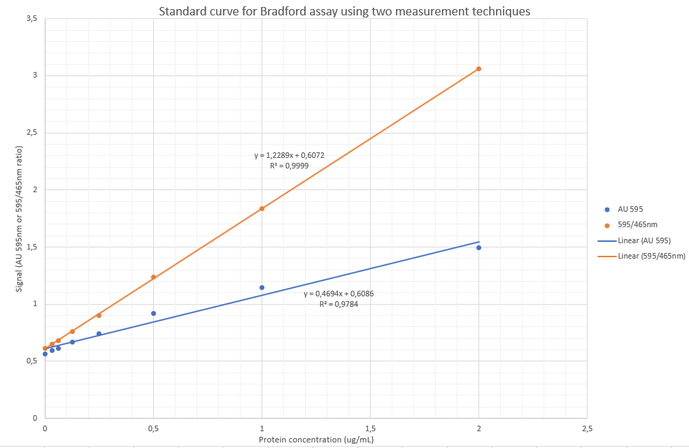
Table 1 – Absorbance values obtained
To determine the unknown:
Via AU595nm:
y=0.4694x + 0.6086
x= (y-0.6086)/0.4694
x= 1.34g/L
Via the 595/465nm ratio:
y = 1.2289x + 0.6072
x=(y-0.6072)/1.2289
x= 1.25g/L
QUESTION 2 (Total 10) Calculate the percentage (%) change over time of your unknown sample and comment on the stability of your assay.
Referring to Fig. 2 – To calculate the %change over time is relatively simple by using the slope of the linear regression line: If using the orange line’s formula at 595nm only: slope = – 0.0081, which means that the absorbance values decreases in general by 0.0081 AU per minute. This is, however subject to variability as the reagent/protein complexes was observed as precipitating out and the final portion of the curve (after 50 min) is likely not fitting due to this phenomenon. Nevertheless, using a decrease of 0.0081AU per minute, means that at an absorbance value of 1.25 (top of the calibration curve),
0.0081/1.25*100 =
0.65% decrease in absorbance per minute.
The stability of the assay is likely around 15-20 minutes.
QUESTION 3 (Total 15) Calculate the CV% and SD using your data.
Absorbance Value
Calculation
1.6096
1.6124
1.5923
1.5345
1.498
1.5602
1.5624
1.5425
1.4823
1.4567
Stdv
0.050538
Mean ( (Sum of values)/n)
1.54509
CV%
3.270859 %
Calculation of mean absorbance and CV on the highest standard.
QUESTION 4 (Total 10) Calculate the LOD, LOQ, and comment on the linearity of your assay.
Using only the 595nm absorbance yielded a poor result (r=0.9784).
Using the 595/465 ratio, the linearity was much better (r = 0.9999)
SE of intercept: Excel Function: STEYX(X-values;Y-values)
LOD = 3.3 * (SD of intercept / slope)
LOQ = 10 * (SD of intercept / slope)
Prot. Conc
Abs 595
465nm
595/465 ratio
2
1,4949
0,488
3,06332
1
1,146
0,6248
1,834187
0,5
0,9158
0,7388
1,239578
0,25
0,7401
0,8203
0,902231
0,125
0,6648
0,8788
0,756486
0,0625
0,6138
0,9023
0,680262
0,03125
0,5932
0,9143
0,648802
0
0,5633
0,9234
0,610028
AU595 only
Slope
0,469384
STEYX
0,052252
LOD
0,367358
ug/mL
LOQ
1,113206
ug/mL
595/465 ratio
Slope
1,228876
STEYX
0,051192
LOD
0,137467
ug/mL
LOQ
0,416565
ug/mL
Table 2 – Limit of detection (LOD) and limit of quantification (LOQ) between the different measuring procedures.
REFERENCES: Becker, J. M., Caldwell, G. A. and Zachgo, E. A. (1996) ‘Protein Assays’, in Biotechnology. Elsevier, pp. 119–124. doi: 10.1016/b978-012084562-0/50069-2. Bradford, M. M. (1976) A Rapid and Sensitive Method for the Quantitation of Microgram Quantities of Protein Utilizing the Principle of Protein-Dye Binding, ANALYTICAL BIOCHEMISTRY. Kruger, N. J. (2009) ‘The Bradford Method For Protein Quantitation’, in The Protein Protocols Handbook. Humana Press, Totowa, NJ, pp. 17–24. doi: 10.1007/978-1-59745-198-7_4. Nouroozi, R. V. and Noroozi, Moulood Valipour Ahmadizadeh, M. (2015) ‘Determination of Protein Concentration Using Bradford Microplate Protein Quantification Assay’, International Electronic Journal of Medicine, 4(1), pp. 11–17. doi: 10.31661/iejm158.