Total Protein assay – Bradford
Practical 3 :
PROTEIN ASSAY- BRADFORD
Total /100
INTRODUCTION
The Bradford protein assay, is a spectrophotometric assay that is more popular for protein concentration determination than other known protein assay such as the Lowry assay. The Bradford assay is simple, more sensitive and faster than other protein assays (Kruger, 2009). This assay is an example of a dye-binding assay and the dye used is Coomassie Brilliant Blue G-250 (Bradford, 1976; Becker, Caldwell and Zachgo, 1996; Kruger, 2009; Nouroozi and Noroozi, Moulood Valipour Ahmadizadeh, 2015). The principle of this assay relies on the physical interaction of the dye and protein in solution and results in an observable change in colour. The colour change is as follows; red (Amax 465 nm), when not bound to proteins and blue (Amax 595 nm) form of the dye carries a (-) charge and interacts with (+) charges on proteins to form a complex (Becker, Caldwell and Zachgo, 1996).
OBJECTIVES
2.1. To prepare standards through a series of dilutions
2.2. To measure the unknown concentration of a protein in solution via a spectrophotometer
2.3. To analyse, interpret results about CV%, SD, LOD and LOQ.
PROCEDURES
A. PREPARATION BEFORE THE PRACTICAL
Complete the following BEFORE your practical session:
• You would need to do some extra reading on the Bradford protein assay and spectrophotometer principles (i.e. Beer Lambert law) in preparation for your practical and test.
• Find and print SDS’s for the following chemicals; Tris (trisaminomethane), Hidrochloric acid (HCL), ethanol, Phosphoric acid and Coomassie Brilliant Blue G-250.
• Prepare a practical plan for your experiment that you will be conducting today.
B. PRACTICAL SESSION (Total 50)
Complete the following DURING your practical session:
(1) Complete the practical test.
(2) Using the Bradford Assay determine as follows:
Materials provided:
• Tris buffer: 10 mM Tris-HCl (pH 7.0)]
• Bovine serum albumin (BSA) stock solution: [2 mg/ml BSA in Tris buffer (pH 7)]
• Bradford reagent; [0.01% (w/v) Coomassie Brilliant Blue G-250, 4.7% (w/v) ethanol, 8.5% (w/v) phosphoric acid]
• Unknown protein sample
Method:
a) In Eppendorf tubes, prepare a series of BSA solutions of varying concentration by diluting the
2 mg/ml BSA stock solution with Tris-HCL buffer (You will need ~200μL of each dilution) to set up a calibration curve (at least 7 concentrations to be used).
Serial dilutions were made in 1.5mL Eppendorf tubes:
| Standard no. | Protein concentration (ug/ml) |
| 1 (500uL of provided 2ug/ml stock solution) | 2 |
| 2 (250 uL of S1 plus 250uL Tris-HCl diluent) | 1 |
| 3 (250 uL of S2 plus 250uL Tris-HCl diluent) | 0.5 |
| 4 (250 uL of S3 plus 250uL Tris-HCl diluent) | 0.25 |
| 5 (250 uL of S4 plus 250uL Tris-HCl diluent) | 0.125 |
| 6 (250 uL of S5 plus 250uL Tris-HCl diluent) | 0.0625 |
| 7 (250 uL of S6 plus 250uL Tris-HCl diluent) | 0.03125 |
| 8 (Also Blank – Only 250uL Tris-HCl) | 0 |
b) Add 2.5 mL of Bradford reagent to a separate cuvette for each of your samples and label them appropriately. Consider the value of determining the concentration of one or more dilutions of your unknown sample as well as the undiluted (“neat”) unknown sample.
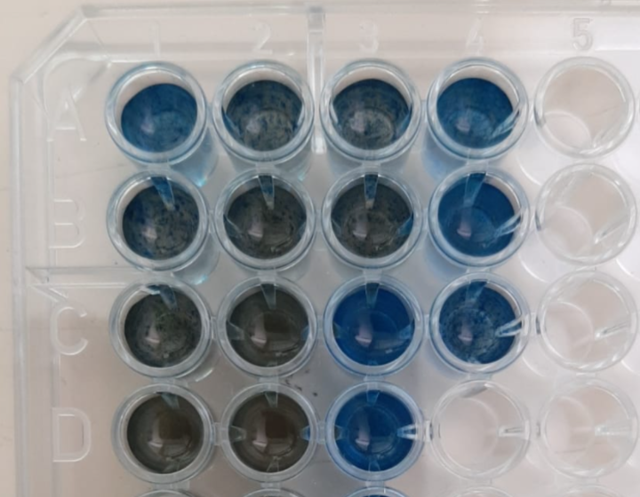
To save cuvettes, I have used an old refurbished microtitre plate with 10x less volume, hence 250uL
c) Prepare your samples by adding 50μL of each protein sample (diluted standard or unknown) separately to the Bradford reagent in the appropriately labelled tube. Mix the tubes by gentle inversion several times, and let the colour develop for 5 min. Observe and record the colour change of your standard samples as a function of protein concentration. A blank sample is prepared by mixing 50μL Tris buffer with 2.5 ml Bradford reagent.
As above, to save reagent and test my pipetting skills, I have used 5uL as one set of additions and also made a 1:1 (2x) dilution of my standards to run another calibration curve. The unknown sample was also added as neat and a 2x dilution.
d) You will need to determine which portion of the UV/vis spectrum, specifically which wavelength will be useful for following the dye bound by protein. Take a full spectral scan of your Bradford reagent blank. When your standard samples have fully developed, take a full spectral scan of the most concentrated standard you prepared.

e) Based on your results, choose a single wavelength suitable to analyse the results of your dye-binding assay. Measure and record the absorbance of each standard and unknown sample at your chosen wavelengths using cuvettes.
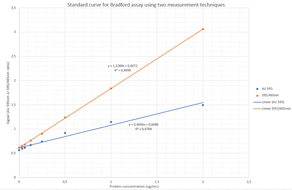
From above wavelength scan it is evidenced that the maximum absorbance after colour development occurs at 595 as published widely in the literature for the Bradford assay. I am, however going to perform a slight variation also published before, by using the ratio of absorbance 595nm/465nm as the signal, as it has before been shown to be more sensitive. The rationale thereof is that there is reduction of absorbance intensity at 465nm and increase of intensity at 595nm, hence likely causing slight increases in sensitivity and arguably a more accurate assay.
f) At your determined wavelength, read your unknown sample at approximately every 10 minutes for 1 hour, you will use these readings to calculate the percentage (%) change over time.

g) Prepare your highest standard in five (5) cuvettes and read the absorbances of each cuvette two times, so in total you will have 10 readings. These results you will use to calculate the protein concentrations and then calculate the CV% and SD
h) Make sure your lab space is clean and disinfected.
C. AFTER PRACTICAL SESSION
Complete the following for submission before or during the next practical
Answer the following questions:
QUESTION 1 (Total 15)
Using the resulting equation for the calibration curve, determine the protein concentration of your unknown sample.
| Prot. Conc | Abs 595 | 465nm | 595/465 ratio |
| 2 | 1,4949 | 0,488 | 3,06332 |
| 1 | 1,146 | 0,6248 | 1,834187 |
| 0,5 | 0,9158 | 0,7388 | 1,239578 |
| 0,25 | 0,7401 | 0,8203 | 0,902231 |
| 0,125 | 0,6648 | 0,8788 | 0,756486 |
| 0,0625 | 0,6138 | 0,9023 | 0,680262 |
| 0,03125 | 0,5932 | 0,9143 | 0,648802 |
| 0 | 0,5633 | 0,9234 | 0,610028 |
To determine the unknown:
Via AU595nm:
y=0.4694x + 0.6086
x= (y-0.6086)/0.4694
x= 1.34g/L
Via the 595/465nm ratio:
y = 1.2289x + 0.6072
x=(y-0.6072)/1.2289
x= 1.25g/L
QUESTION 2 (Total 10)
Calculate the percentage (%) change over time of your unknown sample and comment on the stability of your assay.
Referring to Fig. 2 – To calculate the %change over time is relatively simple by using the slope of the linear regression line: If using the orange line’s formula at 595nm only: slope = – 0.0081, which means that the absorbance values decreases in general by 0.0081 AU per minute. This is, however subject to variability as the reagent/protein complexes was observed as precipitating out and the final portion of the curve (after 50 min) is likely not fitting due to this phenomenon. Nevertheless, using a decrease of 0.0081AU per minute, means that at an absorbance value of 1.25 (top of the calibration curve),
0.0081/1.25*100 =
0.65% decrease in absorbance per minute.
The stability of the assay is likely around 15-20 minutes.
QUESTION 3 (Total 15)
Calculate the CV% and SD using your data.
| Absorbance Value | Calculation |
| 1.6096 | |
| 1.6124 | |
| 1.5923 | |
| 1.5345 | |
| 1.498 | |
| 1.5602 | |
| 1.5624 | |
| 1.5425 | |
| 1.4823 | |
| 1.4567 | |
| Stdv | 0.050538 |
| Mean ( (Sum of values)/n) | 1.54509 |
| CV% | 3.270859 % |
QUESTION 4 (Total 10)
Calculate the LOD, LOQ, and comment on the linearity of your assay.
Using only the 595nm absorbance yielded a poor result (r=0.9784).
Using the 595/465 ratio, the linearity was much better (r = 0.9999)
SE of intercept: Excel Function: STEYX(X-values;Y-values)
LOD = 3.3 * (SD of intercept / slope)
LOQ = 10 * (SD of intercept / slope)
| Prot. Conc | Abs 595 | 465nm | 595/465 ratio |
| 2 | 1,4949 | 0,488 | 3,06332 |
| 1 | 1,146 | 0,6248 | 1,834187 |
| 0,5 | 0,9158 | 0,7388 | 1,239578 |
| 0,25 | 0,7401 | 0,8203 | 0,902231 |
| 0,125 | 0,6648 | 0,8788 | 0,756486 |
| 0,0625 | 0,6138 | 0,9023 | 0,680262 |
| 0,03125 | 0,5932 | 0,9143 | 0,648802 |
| 0 | 0,5633 | 0,9234 | 0,610028 |
| AU595 only | |||
| Slope | 0,469384 | ||
| STEYX | 0,052252 | ||
| LOD | 0,367358 | ug/mL | |
| LOQ | 1,113206 | ug/mL | |
| 595/465 ratio | |||
| Slope | 1,228876 | ||
| STEYX | 0,051192 | ||
| LOD | 0,137467 | ug/mL | |
| LOQ | 0,416565 | ug/mL |
REFERENCES:
Becker, J. M., Caldwell, G. A. and Zachgo, E. A. (1996) ‘Protein Assays’, in Biotechnology. Elsevier, pp. 119–124. doi: 10.1016/b978-012084562-0/50069-2.
Bradford, M. M. (1976) A Rapid and Sensitive Method for the Quantitation of Microgram Quantities of Protein Utilizing the Principle of Protein-Dye Binding, ANALYTICAL BIOCHEMISTRY.
Kruger, N. J. (2009) ‘The Bradford Method For Protein Quantitation’, in The Protein Protocols Handbook. Humana Press, Totowa, NJ, pp. 17–24. doi: 10.1007/978-1-59745-198-7_4.
Nouroozi, R. V. and Noroozi, Moulood Valipour Ahmadizadeh, M. (2015) ‘Determination of Protein Concentration Using Bradford Microplate Protein Quantification Assay’, International Electronic Journal of Medicine, 4(1), pp. 11–17. doi: 10.31661/iejm158.
Raw data: